Capacity Planning Basics Part 1 of 2

The following article has been authored by Blair McGavin and is part 1 of a 2 part series. If you don’t know who Blair is then check out his LinkedIn profile or his contact details are the bottom of this post feel free to reach out. He recently wrote a very thought provoking article on the future of WFM systems – if you have not already read this then worth checking it out, you can find it in the following link – What is the future of wfm systems?. Both myself and Blair welcome your thoughts and comments we would love to hear from you. – Doug Casterton

Capacity Planning – ‘Piece of Cake’

Figuring out how we capture and model all of these data to forecast our service levels and determine our true FTE requirements – otherwise known as Capacity Planning (CP) – that’s my passion. I think I am drawn to this discipline because is has proven to be so difficult for the WFM industry to figure out. On the surface, it seems pretty strait forward. There are four basic pieces of data in our models (volume, Handle Time, Occupancy and Shrinkage / or Utilization. Slap those numbers into some formulas, and there you have it – we need 150 FTE to meet SL’s next month.

Not so fast. I’ve been at this for about 25 years, and I have never seen two analysts or companies do it the same way. So, if we are all using different assumptions, different definitions, and slightly different formulas – and clearly coming up with different answers: Is any of us correct, or are we all correct? And is there a way for us to prove to ourselves we are doing CP correctly? In Engineering school, If I was taking an exam and either used a wrong formula, wrong coefficient, or skipped a step – I came up with the wrong answer, and I lost 10 pts on that part of the exam. So, are all of ‘our’ varied CP methods correct? Nope. Is there a way to prove to ourselves that our methods are solid? Yes! More on that at the end.

Isn’t LinkedIn great! Having a powerful network can be an amazing asset to help advance our careers. But don’t you find the ‘endorsement’ process to be a little humorous. Select a skill, get a few people to endorse that skill, and now you are an industry expert. I have been endorsed by dozens of people for skills for which I have very little experience. But the WFM skill that I think I am most proficient at is Capacity Planning, yet only 2 people have endorsed me for that skill. How is that possible? Those in my network who are close to me and know about my career, know that my CP skills are at the top of my skill set. But still only two endorsements.

I think that observation is indicative of the problem. I believe that there is a perception that if your company/WFM team has ‘a’ Capacity Plan, you therefore have an ‘accurate’ capacity plan. Anyone can do it. It is a commodity that doesn’t require any specialized skills. From my experience, that’s just not true. And you are certainly not going to get the right answer from your WFM software – don’t get me started on this one – I see a therapist who helps we work through these deep-seated frustrations. The key is learning to manage your expectations – the fewer you have of your WFM software, the less therapy you will need. ????

Let’s review the ABC’s of CP

There is a basic formula at the root of our capacity plan that tells us what our FTE requirements will be. The hard part is figuring out what the correct value is for each of these variables:

Ok – let’s call it the ABC’s and D of CP. This is a real basic formula that all of us can remember as we build out the models that help us understand the value of each. Here is what each variable represents:

Volume = A
Productivity = B
Occupancy = C
Utilization = D

So, expanding this out a little bit, we get the following:

There is also another factor in the denominator that sinks up with our volume. If we are using ‘weekly’ volume, then we would have a factor of 40 hours in the denominator – assuming that 1 FTE works 40 hours of regular shift time during a week. Utilization is the inverse of ‘shrinkage,’ which we will discuss later.

Note: It is possible to derive your FTE requirements using multiple steps in your maze of spread sheets, as long as the integrity of this formula is not compromised.

Which of these variables do you think will pose the biggest challenge to figure out? From an effort perspective, accurately tracking your shrinkage will require the most time and effort. Occupancy will require some unique modeling techniques. Volume and HT are a little more strait forward, but still require some thought before inserting values into this formula.

Now, let’s take a deeper dive into some of the challenges we face in determining the correct values for each of these variables.

Occupado – The hotel is full

Why is Occupancy even a part of this equation? Simple math tells us that if I have 1,000 phone calls to answer, and our HT is 6 min (10 calls per hour), we can do the math and figure out that we need 100 hours of work done to answer those calls [ 1000 calls / (10 calls/hr)] = 100 hours. Occupancy tells us how much of our agents’ phone log-in time is busy speaking with customers (Talk time + ACW). An agent with 90% occupancy, had 10% idle time in between calls.

Why do we have to account for Occupancy and add additional time to our staffing models in order to meet service level targets? It’s because we are managing a ‘real-time’ process. Real-time processes don’t behave like a back-office activity. There is variability in the behavior of how customers arrive and are processed within the system: how calls arrive (uniformly or some funky distribution like Poisson), How many calls arrive relative to our forecast, and how long the call occupies an agent – one call might be only 2 minutes and the next call might be 9 min. These two variables are assumed to follow an exponential distribution.

The Erlang formulas try to help us quantify the variability in the process and tell us what our occupancy will be in order to meet SL’s. Figuring out our ‘true’ occupancy at Service Level is the ‘Holy Grail’ in this entire process. Variability is the enemy. The more variability we have, the less efficient we will be and it will drive down our occupancy and increase our staffing. Refer to the ‘professionally’ modeled graph below:

At low volumes there is a LOT of variability in how many calls will arrive which drives down our occupancy. At high volumes, the process behaves much more predictably, both from how many calls will arrive relative to the forecast, AND what our average HT will be. The latter means that the process will be more predictable which will translate to a higher occupancy and higher productivity. This is similar to the concept of ‘risk pooling’ variance. This principle of managing variability is used in Inventory Management and in the financial markets with buying a Mutual Fund instead of individual stocks.

Deriving Occupancy

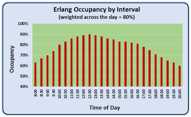
If we were able to display our forecast occupancy (at service level), based on the occupancy values per the Erlang formula, it would look something like the graph below. And then if we took a true weighted average calculation across all of the intervals in the day and came up with an occupancy value of 80% – Is that the value that we would want to use in our Capacity Plan? (this is assuming Erlang is correct – which it ain’t).

The answer is ‘NO.’ There is another issue at play here, and that is our ‘schedule efficiency.’ Poorly aligned schedules will cost us more resulting in lower occupancy.

So how can we account for all of the flaws in Erlang and ALSO quantify the inefficiencies in our schedules? There is a fairly easy modeling trick that will give us the answer.

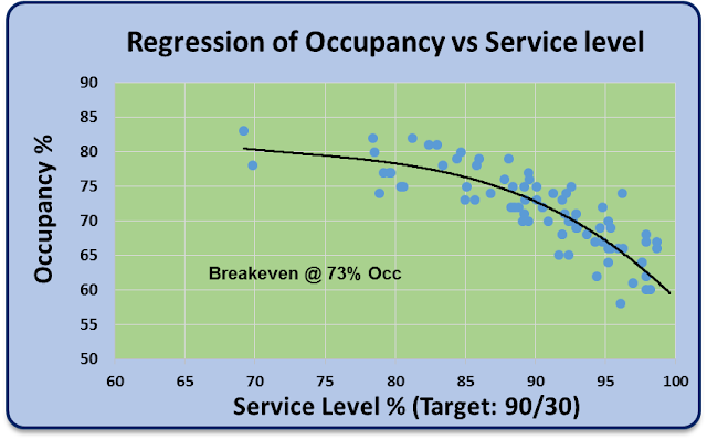
We can build a scatter plot of our ACD data, and it will give us the answer we are looking for . The two variables that we are interested in plotting against each other are: 1) Occupancy and 2) Service level. The SL could either be ASA or SL % in XX seconds. There are 3 different levels at which you could possibly model your ACD data: Interval, Daily, or Weekly.

For this exercise, you want to look at your Dailyresults. There are a few tricks to building these scatter plots, but hopefully it’s pretty strait forward.

· – You will want to use 2-3 months of recent data

· – Manually remove or delete data points that are obvious outliers.

· – If certain days of the week (like the weekends), have noticeably different volumes – you will want to build separate models: 1 for Mon – Fri, and a 2^nd for Sat / Sun. Remember Occupancy is volume sensitive, so you would come up with two different answers.

In the example above, the breakeven point for the SL target of 90% of calls answered within 30 seconds – is at 73% occupancy => (.73) is the value you would use in our standard CP formula for occupancy. This method is a far-cry from having an accurate substitute to replace Erlang for interval level forecasting, but it will get the job done for high level capacity planning.

As mentioned at the start of this article this is the first part of a two part series on capacity planning. Part 2 will cover everything from Shrinkage, handle times, and Tom Cruise in Mission Impossible, the aim is to have part 2 posted this coming Sunday. If you have not already subscribed by email to this blog, then be sure to do so, in order not to miss out on part 2 and future weekly articles.

May the FORCE be with you, and a LOT of luck.

Once again, Doug and I welcome your thoughts and comments.

Blair McGavin

Email: blairmcgavin@msn.com

https://www.linkedin.com/in/blair-mcgavin-3b97542