Contact Center Basic Forecasting Building Blocks

The basic building blocks of a systematic forecasting approach (Systematic: Components of the time series that have consistency or recurrence and can be described and modelled) can be based on relatively simple mathematical methods.
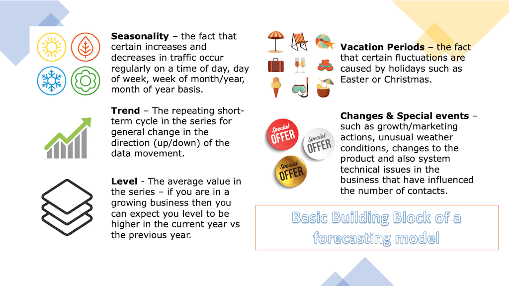
Daily, Weekly, Monthly Volume forecasting involves thinking of a series as a combination of level, trend, seasonality, and noise components in addition to the Poisson fluctuations that you can expect. These components for a customer operational forecast have been depicted above.
Simply put, to be able to predict the future we need to first understand what has occurred previously and extrapolate that into the future. Thus, analysing the historic volume and explaining what has occurred using these factors above are perhaps the most critical part of any forecasting process. Analysing the influence of these factors one by one is known as a decomposition method.
Making a graphical plot of the data actuals available is often not that insightful due to the weekly cycle and special events that are likely to mask the identification of a slight but steady increases in contact volume. For example, we usually can quite clearly see the weekly cycle, with less traffic on Saturday and Sunday vs a weekday – often with the Monday as the highest volume day. However, it is often difficult to identify all outliers in order to derive a trend. It is for this reason, we have to identify the special events and holidays and then deseasonalize the data. This should be done for the weekly cycle, but can also be completed for the yearly cycle if enough data is available.
In a perfect world following deseaonalizing we would get a straight line representing the long-term trend, with special days and the seasons filtered out. Of course if after this effort the line was representing a flat profile, then there is no trend. However, we rarely get such a flat profile and there will still be unexplained variations. Some of these will be caused by normal Poisson fluctuations, but often they are bigger than we would expect just from a Poisson distribution. Once you have identified the trend you can start to assemble the forecasting.
Once the trend is determined we can now include the seasons (both intra-week and intra-year) and then the special days to produce the forecast. While deseasonalizing consisted of dividing by the average per day or week, seasonalizing consists of multiplying the deseasonalized forecast by the seasonal factors. To correct the forecast for special days and events we have to quantity their effect. This can be achieved via various methods, but even simple averaging can effective as a method, if past events are likely to be similar to future one.
So this concludes a brief overview of a very simple but effective forecasting method. It should be noted that there are many elements that need to factored and they will vary from operation to operation. For example, things that are likely to differ from operation to operation are; the amount of available data, the volatility of that data, and the extent to which special days influence.
Thus, the only way to decide on what to include and what not to include is to test continually using a systematic approach of continuous improvement.
For further reading on the Contact Center Forecasting topic, check the following out:
Volume Demand Forecasting – introducing some more slightly more advanced topics
Time-Series Forecasting – some common methods used.
Forecasting Accuracy Targets – key considerations when looking to measure forecast accuracy
Methods to Measure Forecast Error – The first rule of forecasting is that all forecasts are either wrong or lucky.
Smoothing Spline – It is really possible to make intra-day patterns better and easier


Responses