Hello, Welcome All. In this article we will look at the different Models of Time Series forecasting which can be done for the data analysis.

Time Series Forecasting – Exercise 1

We are going to look at certain Simple Forecasting Methods as shown below 1. Naive Method 2. Seasonal Naive Method 3. Random Walk with Drift

The models will be explained in detail along with the formula and actual forecast data for our sample series data.

We have a sample series data of sales from a FMCG company from 2002 to 2016 on a quarterly basis

So, lets begin!!

Step 1: Install the Required Packages in R and Load them

#install.packages(“smooth”)
#install.packages(“Mcomp”)
#install.packages(“forecast”)
pacman::p_load(pacman,dplyr,GGally,ggplot2,ggthemes,ggvis,
httr,lubridate,plotly,rio,rmarkdown,shiny,stringr,tidyr)

# To load the data

library(“smooth”)

## Loading required package: greybox

## Registered S3 method overwritten by ‘quantmod’:
##   method            from
##   as.zoo.data.frame zoo

## Package “greybox”, v0.6.0 loaded.

##
## Attaching package: ‘greybox’

## The following object is masked from ‘package:tidyr’:
##
##     spread

## The following object is masked from ‘package:lubridate’:
##
##     hm

## This is package “smooth”, v2.6.0

library(“Mcomp”)

## Loading required package: forecast

library(“forecast”)

Step 2: Load the Sample Data in R using the below program

library(readxl)
mydata <- read_excel(“D:/WFM Guru/Forecasting Techniques/Time Series/Data File.xlsx”)

Step 3: Create a Time Series from the loaded Data

myts <- ts(mydata, start = c(2002,1), frequency = 4)

Note: The Frequency is set to 4 which represents the data being in quarterly format

Naive Forecasting Method

Naive consists of the forecast equal to the previous period data.

The formula is:

naivefc <- naive(myts, h=8)
summary(naivefc)

##
## Forecast method: Naive method
##
## Model Information:
## Call: naive(y = myts, h = 8)
##
## Residual sd: 443.0772
##
## Error measures:
##                    ME     RMSE     MAE       MPE     MAPE     MASE       ACF1
## Training set 21.47458 439.8308 337.678 -34.57507 85.91998 10.75652 -0.3762134
##
## Forecasts:
##         Point Forecast      Lo 80    Hi 80       Lo 95    Hi 95
## 2017 Q1           1422  858.33415 1985.666   559.94747 2284.053
## 2017 Q2           1422  624.85610 2219.144   202.87362 2641.126
## 2017 Q3           1422  445.70210 2398.298   -71.11879 2915.119
## 2017 Q4           1422  294.66829 2549.332  -302.10507 3146.105
## 2018 Q1           1422  161.60483 2682.395  -505.60807 3349.608
## 2018 Q2           1422   41.30627 2802.694  -689.58884 3533.589
## 2018 Q3           1422  -69.31967 2913.320  -858.77662 3702.777
## 2018 Q4           1422 -172.28779 3016.288 -1016.25277 3860.253

Seasonal Naive Forecasting Method

Seasonal Naive consists of the forecast equal to the previous season data.

The formula is:  , m is the previous season.

snaivefc <- snaive(myts, h=8)
summary(snaivefc)

##
## Forecast method: Seasonal naive method
##
## Model Information:
## Call: snaive(y = myts, h = 8)
##
## Residual sd: 22.4108
##
## Error measures:
##                    ME     RMSE      MAE      MPE     MAPE MASE       ACF1
## Training set 31.39286 38.45498 31.39286 6.315174 6.315174    1 0.04279075
##
## Forecasts:
##         Point Forecast     Lo 80     Hi 80     Lo 95     Hi 95
## 2017 Q1            386  336.7180  435.2820  310.6296  461.3704
## 2017 Q2            448  398.7180  497.2820  372.6296  523.3704
## 2017 Q3            657  607.7180  706.2820  581.6296  732.3704
## 2017 Q4           1422 1372.7180 1471.2820 1346.6296 1497.3704
## 2018 Q1            386  316.3047  455.6953  279.4102  492.5898
## 2018 Q2            448  378.3047  517.6953  341.4102  554.5898
## 2018 Q3            657  587.3047  726.6953  550.4102  763.5898
## 2018 Q4           1422 1352.3047 1491.6953 1315.4102 1528.5898

Random Walk with Drift

Random Walk with Drift Method consists of forecast equal to the previous data plus the arithmetic mean of previous period’s historical data differences.

The formula is: ,  is the arithmetic drift.

rwfc <- rwf(myts, h=8, drift = TRUE)
summary(rwfc)

##
## Forecast method: Random walk with drift
##
## Model Information:
## Call: rwf(y = myts, h = 8, drift = TRUE)
##
## Drift: 21.4746  (se 57.6837)
## Residual sd: 443.0772
##
## Error measures:
##                         ME     RMSE      MAE       MPE    MAPE    MASE
## Training set -1.920309e-15 439.3062 326.3947 -40.60613 84.0758 10.3971
##                    ACF1
## Training set -0.3762134
##
## Forecasts:
##         Point Forecast       Lo 80    Hi 80       Lo 95    Hi 95
## 2017 Q1       1443.475  875.648317 2011.301   575.05925 2311.890
## 2017 Q2       1464.949  655.144831 2274.753   226.46032 2703.438
## 2017 Q3       1486.424  486.389162 2486.458   -42.99716 3015.845
## 2017 Q4       1507.898  343.731243 2672.065  -272.54157 3288.338
## 2018 Q1       1529.373  217.339925 2841.406  -477.20837 3535.954
## 2018 Q2       1550.847  102.225448 2999.469  -664.62872 3766.324
## 2018 Q3       1572.322   -4.545333 3149.189  -839.28849 3983.933
## 2018 Q4       1593.797 -104.863266 3292.456 -1004.07949 4191.673

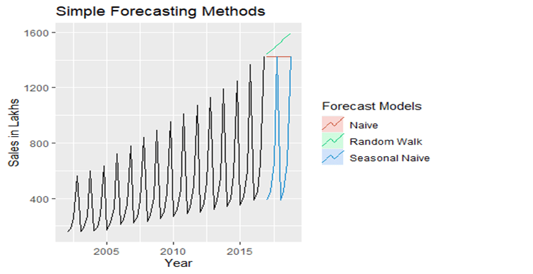
Once we have all the forecast models, let’s plot the graph to visualize the same.

Now, we know how the graphs looks like, but we should be able to decide the best model using the Root Mean Squared Error(RMSE). We can use the below code to find out.

accuracy(naivefc)

##                    ME     RMSE     MAE       MPE     MAPE     MASE       ACF1
## Training set 21.47458 439.8308 337.678 -34.57507 85.91998 10.75652 -0.3762134

accuracy(snaivefc)

##                    ME     RMSE      MAE      MPE     MAPE MASE       ACF1
## Training set 31.39286 38.45498 31.39286 6.315174 6.315174    1 0.04279075

accuracy(rwfc)

##                         ME     RMSE      MAE       MPE    MAPE    MASE
## Training set -1.920309e-15 439.3062 326.3947 -40.60613 84.0758 10.3971
##                    ACF1
## Training set -0.3762134

Conclusion

As we can see, the Seasonal Naive Method has the lowest Root Mean Squared Error (RMSE). Hence it is the best forecasting method for this dataset.

Thank you for Reading????????

Author: Vinay Vasudevan

WFM Data Scientist and WFM Expert

International WFM quiz winner 2020

Stay Tuned!!

Disclaimer: This article is purely my personal view and understanding, this doesn’t depict any organization data